![]() Hello Challengers!
Hello Challengers!
As you work through this challenge, you might be wondering what different kinds of confidence measures you can use with your model results beyond what the team provided in the Starter Notebook. No need to fear, we have some insights that you may find useful for solving the Reflection Connection Challenge.
1. Uncertainty quantification – why is it so hard?
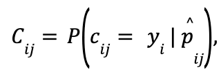
When performing classification with a machine learning approach, you often want to not only predict the class label, but also obtain a probability for the respective label. This probability, associated with each prediction, gives you some kind of confidence in the prediction. It’s important to notice the difference between a model’s probabilistic output and actual model confidence. Let’s assume that for a given i-th observation a model predicts a probability pi of class j. We can then define confidence for this prediction, Cij, as an actual probability of the predicted class belonging to class j:
Where yi denotes actual label of i-th observation and cij stands for each class in the label set allowed for this observation.
Estimating Cij directly is often impossible – however, we can define an estimator that will predict a proxy value of confidence, let’s denote it ![]() The objective of confidence calibration is then to minimize the calibration error – a difference between Cij (unknown) and
The objective of confidence calibration is then to minimize the calibration error – a difference between Cij (unknown) and ![]() In a real-world scenario we can approximate Cij based on true labels by using binning techniques – see Calibration Error — PyTorch-Metrics 1.8.2 documentation for some different definitions of calibration errors.
In a real-world scenario we can approximate Cij based on true labels by using binning techniques – see Calibration Error — PyTorch-Metrics 1.8.2 documentation for some different definitions of calibration errors.
You can use the following implementation of Expected Calibration Error in Python to score your predictions:
def expected_calibration_error(samples: np.ndarray, true_labels: np.ndarray, M: int=10) -> float:
“””
Calculate ECE score over M bins for the selected class
:param samples: array of probabilities for the class
:param true_labels: array of true binary labels (one-vs-all)
:param M: number of bins (keep it constant across you experiments)
“””
    # uniform binning approach with M number of bins
    bin_boundaries = np.linspace(0, 1, M + 1)
    bin_lowers = bin_boundaries[:-1]
    bin_uppers = bin_boundaries[1:]

    # get max probability per sample i
    confidences = np.max(samples, axis=1)
    # get predictions from confidences (positional in this case)
    predicted_label = np.argmax(samples, axis=1)

    # get a boolean list of correct/false predictions
    accuracies = predicted_label==true_labels

    ece = np.zeros(1)
    for bin_lower, bin_upper in zip(bin_lowers, bin_uppers):
        # determine if sample is in bin m (between bin lower & upper)
        in_bin = np.logical_and(confidences > bin_lower.item(), confidences <= bin_upper.item())
        # can calculate the empirical probability of a sample falling into bin m: (|Bm|/n)
        prob_in_bin = in_bin.mean()

        if prob_in_bin.item() > 0:
            # get the accuracy of bin m: acc(Bm)
            accuracy_in_bin = accuracies[in_bin].mean()
            # get the average confidence of bin m: conf(Bm)
            avg_confidence_in_bin = confidences[in_bin].mean()
            # calculate |acc(Bm) - conf(Bm)| * (|Bm|/n) for bin m and add to the total ECE
            ece += np.abs(avg_confidence_in_bin - accuracy_in_bin) * prob_in_bin
    return ece
A valid confidence metric ![]() becomes especially important when it comes to few-shot learning problems where predictions usually come with high uncertainty, varying strongly between classes. We would intuitively expect the model to have more confidence in labeling instances of classes that had sufficient representation in the training set – but at the same time have enough variance to predict minority (or even one-shot) classes.
becomes especially important when it comes to few-shot learning problems where predictions usually come with high uncertainty, varying strongly between classes. We would intuitively expect the model to have more confidence in labeling instances of classes that had sufficient representation in the training set – but at the same time have enough variance to predict minority (or even one-shot) classes.
Overestimating output probabilities is the fundamental problem with classifiers based on neural networks. Essentially two aspects of training contribute to this issue:
- Standard loss functions (like BCELoss) force outputs as close to 0 or 1 as possible.
- Exponential character of output layer activation keeps pushing outputs toward 0 or 1 even when a less strict loss function is used.
There are multiple ways to calibrate output probabilities of neural networks – we will cover two that are widely used: Temperature Scaling and Conformal Prediction. Both techniques require division of the validation data set into two parts: a calibration set, that will be used to train a probabilistic wrapper, and a true test set containing data used to assess quality of calibration.
2. Temperature Scaling
Temperature Scaling is a simple, yet effective technique used to calibrate outputs of the probabilistic output layer by scaling them down. During calibration, a single learnable parameter T is adjusted to “cool down” the outputs (for more details check out the original paper [1706.04599] On Calibration of Modern Neural Networks). Temperature scaling can be used safely in any scenario as it doesn’t affect model accuracy.
You can use the following snippet to set up the Temperature Scaling wrapper (calibrated to minimize Brier score) with AWS Fortuna in just few lines of code:
from fortuna.calibration.binary_classification.temp_scaling.brier_binary_temp_scaling import BrierBinaryClassificationTemperatureScaling

# calib_outputs is an array of probabilities for predicted class
# calib targets is an array of true labels
scaler = BrierBinaryClassificationTemperatureScaling()
scaler.fit(calib_outputs, calib_targets)

# we can now scale model outputs to achieve proper probabilities:
calib_probs = scaler.predict_proba(calib_outputs)
test_probs = scaler.predict_proba(test_outputs)
Temperature Scaling may be a good first step in your calibration pipeline in case you are using a classification model, however due to its uniform treatment of the outputs it won’t affect the order of predictions. It may also be insufficient for minority classes since it assumes a perfect model, where the initial calibration error is independent of both true label and input features. We can intuitively judge that this assumption won’t hold against a few-shot model.
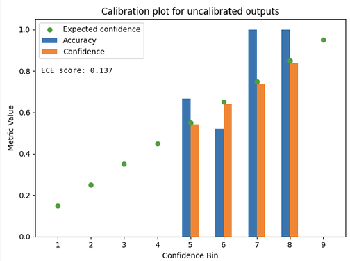
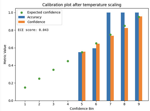
To demonstrate the impact of the technique on model outputs we trained a simple classifier on top of absolute difference between embeddings of image pairs. Charts below show the difference in ECE score and calibration plots between raw model outputs and outputs of temperature-scaled model for the test set:
We can see that after applying Temperature Scaling the predicted probabilities match accuracies within each bin notably more closely compared to the uncalibrated classifier. This is also reflected by the huge drop in ECE score. Perfect calibration should yield the exact match. The slight difference between theoretical and measured confidence within each bin indicates that the confidence distribution within each bin is close to uniform - this allows for the correct approximation of ECE score.
3. Conformal Prediction
Conformal prediction is the model-agnostic approach for model uncertainty quantification. It relies on a simple principle given any proper uncertainty metric of a probabilistic model; we can calibrate it on a separate dataset using conformal transformation. The only assumption for conformal prediction is exchangeability of train, calibration and test data – meaning we can swap any two observations between each other without violating associations within the dataset. The following paper does a great job in explaining basic concepts of conformal prediction:
The greatest advantage of Conformal Prediction is that we can use any metric for initial uncertainty estimates that will be then calibrated. Let’s assume that we have trained a Siamese Neural Network h, that takes a vector of input image features(X1,X2) and outputs their embeddings in latent space Y1,Y2:
![]()
We now need to introduce a nonconformity score, where larger values encode more uncertainty in terms of binary classification. We can define a binary classifier on top of embeddings as a model that outputs 1 where X1,X2 belong to the same class and 0 otherwise. The simplest variation of such a classifier would be a threshold model on distances between the embeddings.
In the starter notebook we already defined the initial quality metric of the model based on a normalized distance between output embeddings. We can then simply use Euclidean distance between images in the latent space as our nonconformity score. The next step would be to account for different probability distributions across different classes. We can resort to unsupervised clustering methods. If we group embeddings of training images into a set of clusters (that doesn’t have to match the number of classes in the training set). We can then use the flexibility of Conformal Prediction to calibrate separate probabilistic wrappers for each cluster id – of course we need to account for the symmetry of inputs (reversed order of input images) and decide which cluster (query or search) should be then used during inference. This approach is a variation of a technique called Mondrian Conformal Prediction and was designed to unify uncertainty estimation when dealing with imbalanced data.
To learn about more advanced approaches such as Full Transductive or Adaptive Conformal Prediction we recommend following materials:
- https://valeman.medium.com/how-to-use-full-transductive-conformal-prediction-7ed54dc6b72b - article about Full Transductive Conformal Prediction
- GitHub - valeman/awesome-conformal-prediction: A professionally curated list of awesome Conformal Prediction videos, tutorials, books, papers, PhD and MSc theses, articles and open-source libraries. - collection of papers, tutorials and Python libraries for Conformal Prediction.
Good luck, we have confidence in your success!
Onward Team ![]()


